Introduction to ANOVA Analysis
Education comes from within; you get it by struggle and effort and thought. – Napoleon Hill
Are you ready to think and struggle through the next topic in the Six Sigma Green Belt Body of Knowledge – ANOVA.
ANOVA stands for ANalysis Of VAriance and it is a hypothesis test used to compare the means of 2 or more groups.
I know what you’re thinking – WHY would we test MEAN VALUES using VARIANCE.
I thought the same thing. . . Don’t worry though.
It’ll all make sense soon!
Ok, so here’s what you’ll learn in this chapter:
- First, we cover the assumptions associated with ANOVA.
- Second are the common terms & definitions within ANOVA (and DOE).
- Third, I start very high level to answer the question – Why Does ANOVA use Variance to Test Mean Values?
- Fourth, we go through the basics of ANOVA including the Sum of Squares, Degrees of Freedom, Mean Squares, F-value.

Then we go into an example of a One-Way ANOVA and use all of the basics we just learned.
Last, but not least I’ll introduce the idea of a Two-Way ANOVA, including new terms and concepts.
Ready to get started?
 Assumptions of ANOVA
Ok, so first things first – ANOVA is a type of Hypothesis Test used to test hypothesis about Mean values.
So, similar to the other Hypothesis Tests we studied, ANOVA analysis is based on the starting assumption that the null hypothesis is true.
Within ANOVA, the Null Hypothesis is always the same – that all of our sample mean values are equal.
Ho: μa = μb = μc = . . . . . . μk
The Alternative Hypothesis is that at least one mean value is different than the rest.
Ha: Not all means are equal
Make Sense?
The other 3 major assumptions for ANOVA are identical to the assumptions associated with the t-test.
Remember that the t-test is used to test the hypothesis that two means are equal, while ANOVA is used to test the hypothesis that 3+ means are equal. So, it’s logical that they would share common assumptions, which include:
- The Population being studied is Normally Distributed
- The Variance is the same between the various treatments (Homogeneity of Variance)
- There is Independence between sample observations
So, your treatment groups must be normally distributed, and the variances between your treatments should be equal and your samples should be independent from each other.
Terminology in ANOVA
Alright, let’ s go deeper with ANOVA and review the common terms and their definitions.
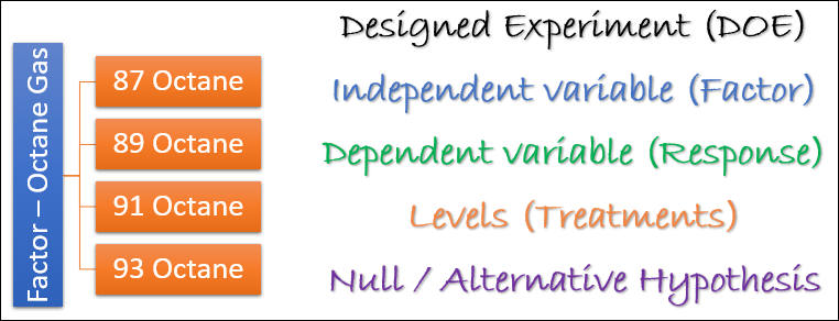
What you’ll often find is that ANOVA Analysis is paired with a Designed Experiment to measure the affect that an independent variable has on a dependent variable.
For example, let’s say you wanted to study the effect that different octane gasses have on the horsepower of your car.
You would design an experiment where you would vary the octane of gas and measure horsepower.

In this experiment, the independent variable would be the octane of gas (87, 89, 91, etc.), and the dependent variable would be the horsepower.
The independent variable in ANOVA is called a Factor.
In the Horsepower example there is only one factor (Octane), which makes this experiment a one-way ANOVA. If there had been two factors (Octane and Fuel Injector Size) it would be a two-way ANOVA.
You’ll notice above that I listed different octanes of gas – 87, 89, 91. These are the different levels or treatments associated with your factor.
So, our Factor (Octane) can have multiple Levels (87, 89, 91) in a One-Way ANOVA analysis.
The Response that we’re measuring in this experiment is Horsepower, which is our dependent variable.
Make Sense? Let’s move on from here to review the basics of ANOVA.
Why Does ANOVA use Variance to Test Mean Values?
ANOVA Takes a very unique and interesting approach to determining if 3 or more sample means all have an equal population mean.
What ANOVA Analysis does – and this is truly brilliant – is it breaks down your data set into two different sources of variation.

When you look at the standard One-Way ANOVA table (Below), you’ll see the two “sources” of variation are called the Treatment and the Error.
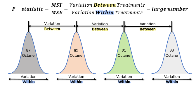
The Treatment Variation is the variability within the data set that can be attributed to the difference between the different treatment groups (difference in sample means).
The Error Variation is the variability within the data set that can be attributed to the random error associated with the response variable. This is the variability within the different treatment groups.
Recall that our null hypothesis within ANOVA is that all population means are equal.
So, if our null hypothesis were true, then we would expect that the treatment variation (difference in sample means) could be fully explained by the random nature of the data.
The treatment variation should be nearly equal to the error variation. This statement is the key to explaining why ANOVA uses Variance to test the difference between Means.

By breaking down our data into the two sources of variance, we can then compare those variances against each of to see if they are statistically significantly different (the alternate hypothesis).
What I’d like to do next is to quickly go through each of the columns of the ANOVA Table and go over each topic specifically.
Including the Sum of Squares and Degrees of Freedom which are combined to calculate the Mean Square Values, which are further combined to calculate your F-Statistic or F-value.
Sum of Squares in ANOVA
Step 1 in the ANOVA process is calculating the Sum of Squares for each of the sources of variation (Treatment & Error), and then adding them up to the total variation within the data set.
The Variation for each of these sources is calculated using the “Sum of Squares” calculation. So, we calculate the Sum of Squares of the Treatment (SSt), and the Sum of Squares of the Error (SSe).
These different sources of variation combine to add up to the Total Sum of Squares (SStotal) within your data set.
Total Sum of Squares (SStotal) = Sum of Square of the Treatment (SSt) + Sum of Squares of the Error (SSe)
Sum of Squares – Example
Ok, let’s go over the formulas to calculate the sum of squares for the treatment, error and then the total sum of squares.
Let’s say we’re back on the horsepower/octane example and we’ve designed an experiment where we’re testing 4 treatment levels (octane levels), and we’re measuring horsepower 10 times per treatment.

So, Treatment group #1 captures our 10 measurements at 87 Octane, and it had a sample mean of 169.7 hp. Make Sense?
Before we calculate the sum of squares, let’s introduce a new topic. The Grand Mean.
So, recall that our null hypothesis is that all three sample means come from the same population mean. If that’s true, we can calculate the Grand Mean, which is an estimate of the population mean.
The Grand Mean for this example is 178.7 hp. You can calculate the grand mean by averaging all of the individual values within the data set.
Sum of Squares of the Treatment
Now we can use the grand mean to calculate the Sum of Squares of the Treatment (SSt).
Recall that the Treatment Variation is the variability within the data set that can be attributed to the difference between the different treatment groups.
We do this by comparing the treatment sample means (X-bar of Treatment Group 1, etc) against the grand mean. We’re also multiplying this difference by “n”, which is the number of samples per treatment group.

Sum of Squares of the Error
Now let’s move on to the Sum of Squares of the Error (SSe).

Remember that the Error Variation is the variability within the data set that can be attributed to the random error associated with the response variable.
This is the variability within the different treatment groups.
So, we’re comparing the individual values (Xi) against that values sample mean (X-bar).
Total Sum of Squares
Now let’s move on to the Total Sum of Squares (SStotal).
We could simply calculate the total sum of squares by adding up the Sum of Square of the Treatment (SSt) and the Sum of Squares of the Error (SSe). Or we could calculate it using the following equation:
This looks similar to the sum of squares of the error calculation; however, we’re now comparing all individual values (Xi) against the grand mean (225).
Let’s compare this to the Sum of Squares of the Treatment and Sum of Squares of the Error:
Total Sum of Squares (SStotal) = Sum of Square of the Treatment (SSt) + Sum of Squares of the Error (SSe)
See how that reconciles?
The total sum of squares captures the total variability within the data set by comparing all values against the grand mean, while the Treatment & Error sum of squares are a unique component of that overall variability.
Alright, so we’ve knocked out the Sum of Squares portion of the ANOVA Table, let’s move on to the Degrees of Freedom column.
Degrees of Freedom in ANOVA
Step 2 in the ANOVA process is to calculate the degrees of freedom (DF) for each source of variation (Treatment & error), which add up to the total degrees of freedom.
We will use the degrees of freedom to “normalize” the sum of squares data to convert the raw “variation” into estimations of the population variance in step 3 (Mean Squares).
So, we will start by calculating the total degrees of freedom (DFtotal) associated with the entire sample data set.
DFtotal = DFerror + DFtreatment
Then we will break this down into the degrees of freedom for the treatment (DFtreatment), and the degrees of freedom for the error (DFerror).
The Total Degrees of Freedom is the easiest to calculate – It’s the total number of observations within your data set, minus 1. The letter N is often used to represent the total number of observations within a data set.
DFtotal = N – 1
The DF of the Treatment is the next easiest to calculate – It’s the number of treatments minus 1. The letter “a” is often used to denote the number of treatments, but this can vary between textbooks.
DFtreatment = a – 1
The DF of the Error is often calculated by taking the total degrees of freedom, and subtracting the treatment degrees of freedom.
DFerror = DFtotal – DFtreatment = (N-1) – (a-1)
Where N equals the total number of observations, which can be calculated as n(a), which is the number of treatment groups (a) times the number of samples per treatment group (n). Using this transformation of N=n*a, we can re-arrange the equation to this:
DFerror = a(n-1)
Ok, before we move on to the next section, let’s take a look at our ANOVA table to see how we’ve incorporated all we’ve learned so far.
So, for the Treatment and Error we’ve calculated the Sum of Squares for each and the Degrees of Freedom for each.
Now it’s time to use that information to move to step 3 in the ANOVA process, calculating the Mean Squares.
Mean Squares in ANOVA
Alright, on to step 3 of the ANOVA analysis, which is the calculation of our Mean Squares, where again we’ll calculate a Mean Square of the Treatment (MST), and a Mean Square of the Error (MSE).
Mean Squares are calculated using the equation below:

We take our Sum of Squares and we divide it by our degrees of freedom.
We will do this for both our treatment and error terms.
This might look super familiar to how we calculate sample variance.
I wanted to show you this to make the point that the Mean Square calculation is a calculation of variance!
Specifically, MST & MSE are both unique & different estimates of the population variance associated with our data set.
If our null hypothesis is true then these two estimates of the population variance will be approximately equal.
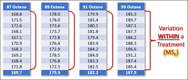
So, the Mean Square of the Error (MSE) is an estimate of the population variance that’s based solely on the variability within each treatment group.
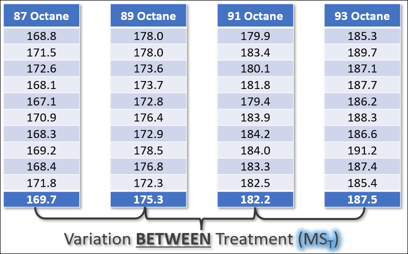
The Mean Square Between Treatments (MST) is an estimate of the population variance that’s based solely on the variability between the treatment group sample means and the grand mean.
Can you see on the left of this image how MST (Mean Square Between the Treatment) is an estimate of the variability between each treatment group and the grand mean?
It compares the sample mean of each treatment to the overall grand mean of the population.
Can you see on the right of this image how MSE (Mean Square of the Error) is an estimate of the variability within each treatment group?
It compares the individual observations within each treatment group, to the sample mean of that treatment group.
Let’s review these two Mean Squares individually.
MSE – The Variability Within the Treatment Groups
The first type of variation measured within ANOVA is the Mean Square of the Error which represents the random variability that is normal to the response variable which.
You’ll see other textbooks call this the Within Treatment Variability because it’s a reflection of the variability within each individual treatment group.
If we go back to our original example of octane & horsepower, you can see that within the 87 octane group, there is some slight variability WITHIN each treatment group.
This random variation in horsepower that’s inherent to each treatment group is the Error Variance.
This next statement is important!
Whether the null hypothesis is true or not, the MSE (Mean Square of the Error) is a good approximation of the population variance.
To calculate the MSE, we use the following formula:
The Mean Square of the Error (MSE) is the Sum of Squares of the Error (SSerror) divided by the Degrees of Freedom of the Error (DFe).
Treatment – The Variability Between the Treatment Groups
The second type of variability within ANOVA is called the MST or Mean Square Between the Treatments and it’s a estimate of the population variance that’s based on the difference between the sample means and the grand mean.
You might also see textbooks call this MSB for Mean Square Between (the treatments), or the Variance Between Treatments because it reflects the variance caused by the different treatments (levels).
This measure of variability compares the sample mean of each treatment (X-bar), against the Grand Mean of the entire sample space (all sample observations).
This next statement is important:
If the null hypothesis is false, then the MST will not be an accurate measure of the population variance.
To calculate the MSE, we use the following formula:
The Mean Square of the Treatment (MST) is the Sum of Squares of the Treatment (SStreatment) divided by the Degrees of Freedom of the Treatment (DFt). In our specific example for octane and horsepower, the MST is:
Now that we’ve calculated both MST & MSE, let’s see what our ANOVA table looks like before we move onto the final step, calculating the F-value.
Comparing the Two Variation Types Against Each Other
Alright, now we’re on to the final step of ANOVA, which is to calculate the F-value associated with our data set, so that we can make an accept/reject decision for our hypothesis test.
Recall that if the null hypothesis is true both MST & MSE will both approximate the population variance, and MST ≈ MSE.
We can compare MST & MSE against each other using the F-test, which is a ratio of the two variances in order to make an accept/reject decision on our null hypothesis.
If the null hypothesis is true and all sample means are equal, then MSE & MST will be approximate equal, and our F-value will equal ~1.
If the null hypothesis is false, and one or more sample groups are not equal to the other sample groups, then MST >> MSE and our F-value will be >>1.
Now, there might be slight differences between MST & MSE which makes MST > MSE, simply due to random chance.
How do we make sure this random variability doesn’t cause us to reject the null hypothesis incorrectly?
This is why we’re using the F-Test, which is a test used to determine the equality of two variances, such as MST & MSE.
The F-Test allows us to determine if our differences between MST & MSE are due to chance or if they are statistically significant.
Many ANOVA tables also include the P-value associated with the F-value. The P-value represents the probability of getting that big of a difference between MST & MSE (or bigger).
This P-value can be compared to your alpha risk to make an accept/reject decision.
If you’re not using a statistical software that gives you a p-value, you can also look up the critical F-statistics in the F-table.
The critical F-statistic is based on your Alpha risk and degrees of freedom for the numerator (MST) & denominator (MSE). Using the example above, the DF of the treatment is 2, and the degrees of freedom of the Error is 6.
The F-Value can then be compared against the critical Fcrit to determine if the calculated Fstat is a statistically significant result.
Below is our ANOVA table with the F-Value.

Two Way ANOVA
How do you feel about One-Way ANOVA?
Are you ready to move on to Two-Way ANOVA?
Before we jump into the differences between One Way and Two-Way ANOVA, it’s important to note that all of the assumptions of One-Way ANOVA apply to Two Way ANOVA.
On to the differences!
So, in One Way ANOVA we were analyzing data that was associated with one single Factor or Independent Variable.
In Two Way ANOVA, we’re going to analyze data where two factors are varied and studied.
In some textbooks you’ll see this as Factor A and Factor B.
Sometimes the second factor is called a “Block”, because you can use it within your experiment to “block” out a certain factor that might be contributing to the error variation.
Similar to One Way ANOVA, Two Way ANOVA allows you to analyze the “main effects” of each factor being varied, by carving out the variation associated with each factor.
This is a new term we haven’t used yet – Main Effects – and it’s meant to denote the variation associated with a single factor. For example, you can have the Main Effects of Factor A, and the Main Effects of Factor B.
When you’ve got two factors, you can also now study the interaction effect between factors. We will talk more about this in the chapter on Designed Experiments.
You can see how the ANOVA table grows in complexity when we move to two factors.
I’ve shown the interactions above, however it’s important to note that if you’re interested in studying the interactions, you must have multiple replicates for each treatment. A replicate is the number of observations per factor.
If you only have 1x replicate (observation) per factor, then there won’t be enough degrees of freedom left over to calculate the interactions effect, and any variability due to the interaction between factors will fall into the error term.
Conclusion
Alright!!! Are you glad that’s done??
Let’s recap quickly.
Ok, so ANOVA stands for ANalysis Of VAriance and it is a hypothesis test used to compare the means of 2 or more groups.
The first we covered are the assumptions associated with ANOVA, which include:
- The Population being studied is Normally Distributed
- The Variance is the same between the various treatments (Homogeneity of Variance)
- There is Independence between sample observations
Second was the common terms & definitions within ANOVA which included Independent variable, dependent variable, factors and treatments (levels).
Third, we answered – Why Does ANOVA use Variance to Test Mean Values?
Then we jumped into the basics of ANOVA including the Sum of Squares, Degrees of Freedom, Mean Squares, F-value.
For the Sum of Squares we reviewed the following equations:
Total Sum of Squares (SStotal) = Sum of Square of the Treatment (SSt) + Sum of Squares of the Error (SSe)
For the Degrees of Freedom we reviewed the following equations:
DFtotal = DFerror + DFtreatment
DFtotal = a*n – 1
DFtreatment = a – 1
DFerror = (N-1) – (a-1) = a(n-1)
We then combined the Sum of Squares and Degrees of Freedom to calculate our Mean Squares.
We then combined MSE & MST into our final calculation of an F-statistic.
To determine if our null hypothesis is true or false, we can compare this F-statistic against a critical F-value from tables.
Looking up this critical value will require you to have an Alpha risk for your hypothesis test and combine that with the Degrees of Freedom for your MST & MSE.
If your f-stat is less than your critical f-value, then you must fail to reject the null hypothesis.
If your f-stat is greater than your critical f-value, then you reject the null hypothesis, and accept the alternative hypothesis that one of the sample means is not equal to the rest.
Lastly, we covered the nuances of going from a One-Way ANOVA to a Two-Way ANOVA.
In Two Way ANOVA we introduced new concepts like Main Effects of factors and Interactions between factors. You can see how the ANOVA table grows in complexity when we move to two factors.