The Normal Distribution is a continuous distribution, and it’s critical in statistics. It’s also commonly referred to as the Gaussian Curve or the Bell Curve due to its symmetric bell shape.
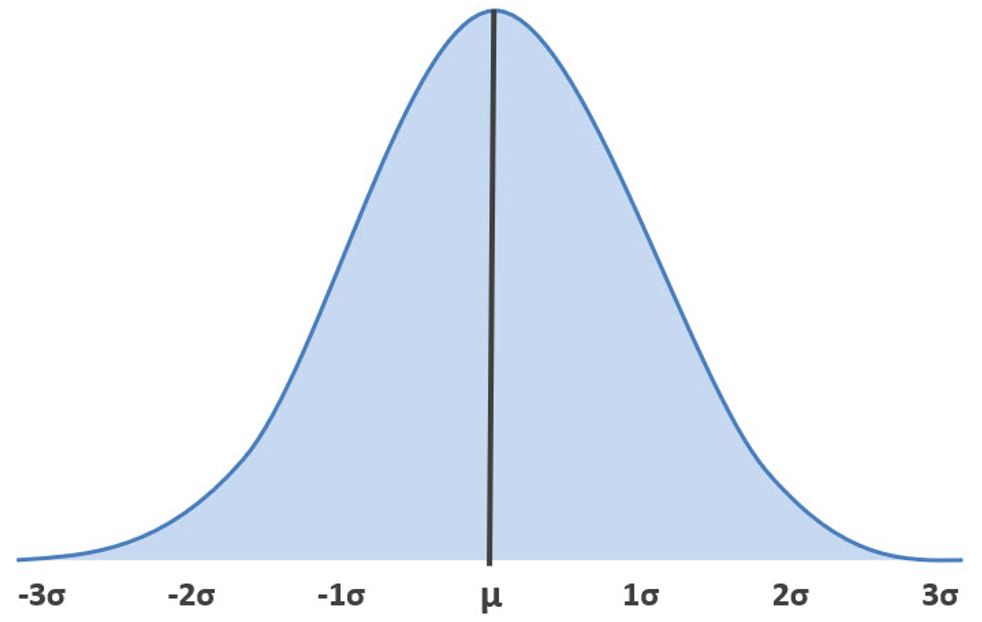
The Normal Distribution is the foundation for many other topics within the Six Sigma Green Belt body of knowledge, such as Process Capability, Statistical Process Control (SPC), Hypothesis Testing, ANOVA Analysis and Linear Regression to name a few. That’s why the normal distribution is super important.
There are two Parameters that fully define this distribution – the Mean (μ) and the Standard Deviation (σ).
The Mean (μ) is a measure of the central tendency of the distribution & often exists at the peak & centerline of the distribution.
The Standard Deviation (σ) is a measure of the variation or spread associated with the distribution.
The shape of the curve is governed mostly by the standard deviation. The smaller the standard deviation, the more data is centered around the mean. When the standard deviation gets bigger, the tails get longer and the data is more dispersed.
The Z-Transformation of the Normal Distribution
Similar to other probability distributions, the area under the normal curve represents the probability of occurrence of X.
To more quickly calculate the area under the normal distribution curve, statisticians have given us the Z-transformation, along with the Z-tables. To perform the Z-transformation, you can use the following equation. This will transform your random variable X, into a Z-value based on the distribution’s mean & standard deviation.
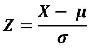
For example, let’s say you’ve got a variable X (Grades on the GB Exam) that follows the normal distribution with a mean value of μ = 82 and a standard deviation of σ = 6. The Z-score for an exam grade of 70 can be calculated as:

We can interpret this result by saying that the exam score of 70 is 2.0 standard deviations below the mean. If you wanted to calculate the proportion of the population which scored less than 70% on the exam, it would look like the gray shaded area below on the distribution: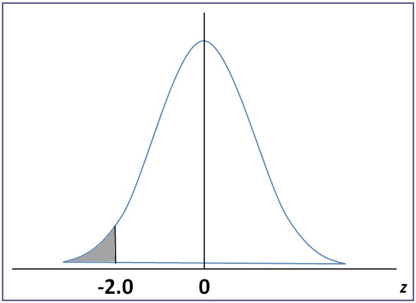
Notice this distribution is not a reflection of the exam score (centered at z=0), but it’s a reflection of the transformed z-score associated with the exam. We can then use the Z-score tables to answer any probability question associated with this value without having to use a calculator.
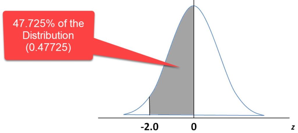
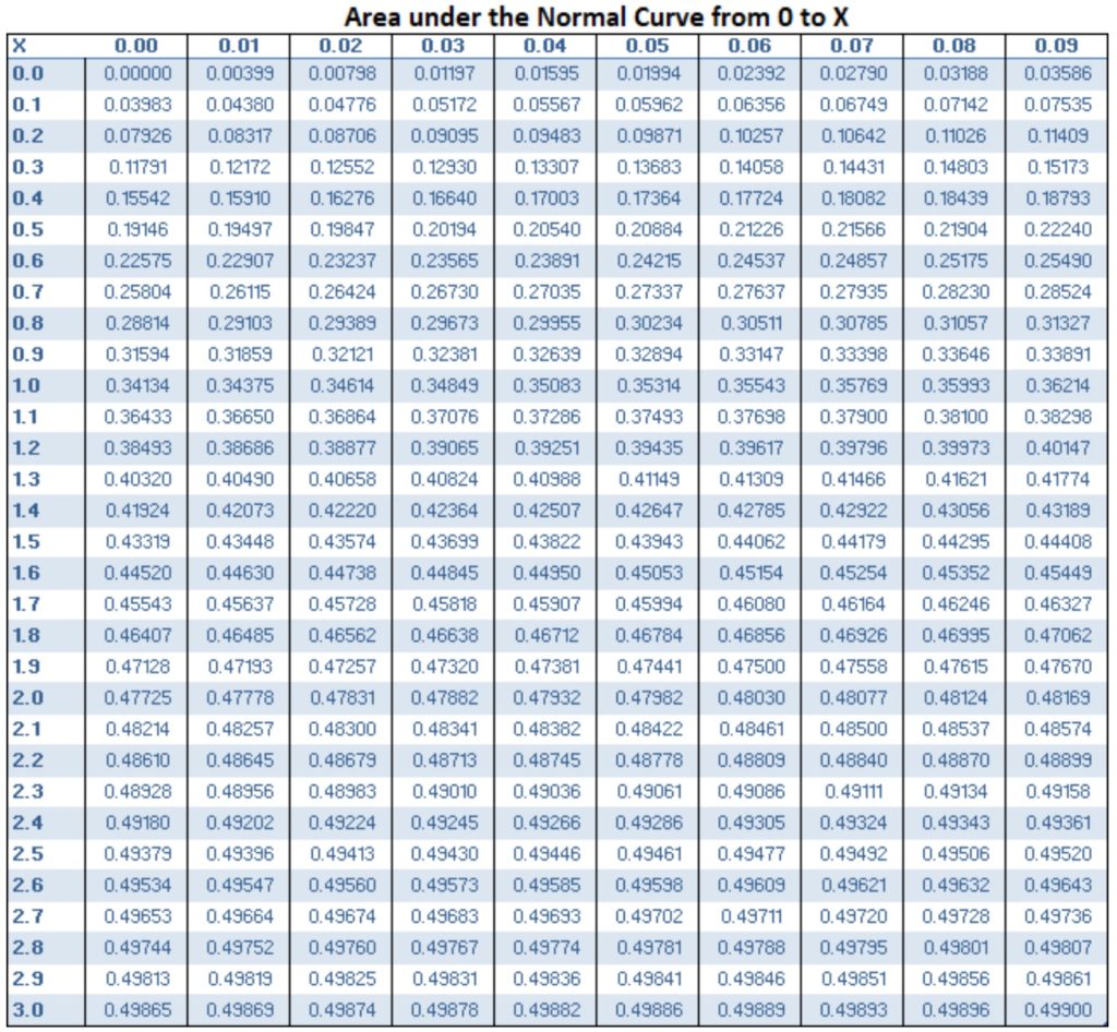
The Z-tables are shown below, and the corresponding probability at a Z= 2.0 is 47.725, which I’ve shown in an updated picture below. Because the normal distribution is symmetric around the mean, that means that 50% of the distribution is on the left half.
So to solve for the area to the left of Z=-2.0, which reflects the percentage of the population of test takers that got a score less than 70, we simply just subtract 47.725 from 50 to get that area of 2.275%.
The Z-Transformation Table of the Normal Distribution
Example Using the Normal Distribution
Let’s do another example of the Z-transformation in a real-life situation. Within the world of Reliability, the normal distribution curve can be used to model the reliability of a system over time.
Let’s say we’re dealing with a motor and we’ve modeled the motors failure over time and it fits the normal distribution. Your test data indicates that the mean and standard deviation associated with the motor is 6,500 hours and 500 hours respectively. What is the reliability (the probability that the motor is still operational) of the motor at 7,200 hours?

Graphically, this looks like:
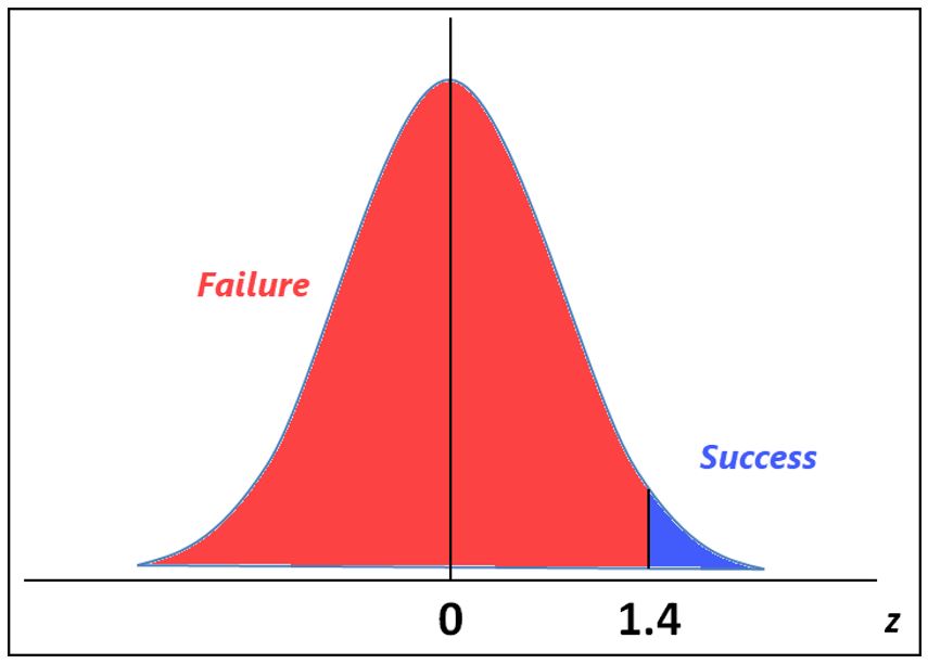
Using the Z-Tables, the area under the curve at Z=1.4 (the area between Z=0 and Z=1.4) is 0.4192, and we add to that the 0.500 that represents the left half of the normal distribution curve, which add up to 0.9192.
Remember that the Z-Score and the resulting probability represent the area to the left of the time value (7,200 hours). So, the reliability is the area to the right of the curve, which is 1 – 0.9192 = 0.0802 = 8.02 %
Therefore, there is nearly an 8% probability that the motor has not yet failed after 7,200 hours. Or, said differently, 8% of the original population of motors are likely still operational after this amount of time.